The Mandelbrot Set

The Mandelbrot set is a famous fractal named after the mathematician Benoit Mandelbrot, who introduced it in a paper in 1980. It is known for its intricate and detailed structure, which is made up of an infinite number of smaller copies of itself. The set has many interesting properties, such as self-similarity and non-differentiability. It is defined by the complex equation $z(n+1) = z(n)^2 + c$, where $z(0) = 0$ and $c$ is a complex number in the form of $a + bi$, where $a$ and $b$ are real numbers. The Mandelbrot set is the set of all complex numbers $c$ for which the sequence $z(n)$ does not diverge to infinity when iterated using the above equation.

The Mandelbrot set is typically visualized by plotting the values of $c$ in the complex plane, and color-coding each point based on how quickly the sequence $z(n)$ diverges. Points that are in the Mandelbrot set are colored black, while those that diverge quickly are colored with bright colors.

You can read more about the Mandelbrot set on this Wikipedia page. The following is code that visualizes the Mandelbrot set using HTML5 and Javascript.

See the Pen The Mandelbrot Set by sherif-gamal (@sgamal) on CodePen.

The code

The code creates a canvas element of size 300x300, and uses the method drawAxes to draw the complex plane.

function drawAxes() {
    ctx.beginPath();
    ctx.moveTo(0, h/2);
    ctx.lineTo(w, h/2);
    ctx.moveTo(w/2, 0);
    ctx.lineTo(w/2, h);
    ctx.stroke();
}

From the linked Wikipedia page

The Mandelbrot set is a compact set, since it is closed and contained in the closed disk of radius 2 around the origin.

Given this fact, we know that the domain for $a$ and $b$ is the interval $[-2, 2]$.

Now, to draw the Mandelbrot set, we need to iterate over every pixel in our 300x300 pixel canvas and:

1. Calculate the corresponding $a$ and $b$ values for the pixel.
2. Iterate the equation $z(n+1) = z(n)^2 + c$ for $n$ from 0 to 1000, and check if the absolute value of $z(n)$ is greater than 2.

To do step 1 we need to apply the transform shown in the following figure:

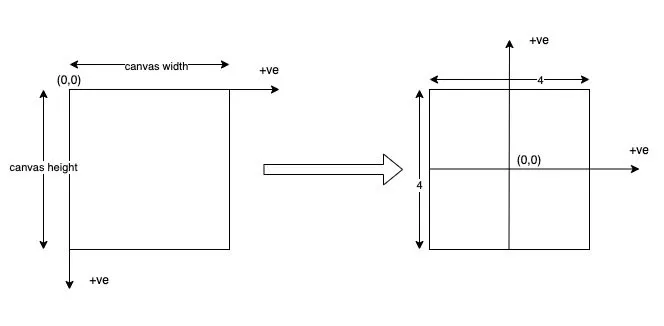
This can be done by applying an affine transformations to each pixel:

where $s_x$ and $s_y$ are the $x$ and $y$ scale factors and $t_x$ and $t_y$ are the translation in $x$ and $y$ respectively. In our case, we want to scale x by a factor of $4/w$ because we want to map our w pixels to the interval $[-2,2]$. Similarly we want to scale y by $4/h$ and invert it i.e. multiply it by $-1$ so that y and b will grow in the same direction (Look at the transformation picture again if confused). Now that we scaled our world from $wxh$ to $4x4$, the mid point which was at $(w/2,h/2)$ is now $(2,-2)$. We can make that $(0,0)$ by adding $(-2,2)$ to it. This gives us the following transformation matrix.

To calculate $a$ and $b$ for a pixel, we use an augmented vector $[x, y, 1]$ and multiply it by the above matrix. This gives us an augmented vector $[a, b, 1]$

Doing this matrix multiplication will result in:

$$a = s_x + t_x$$ $$b = s_y + t_y$$

This means we need to apply the following method to each pixel:

function applyTransform(x, y) {
    const a = 4/w * x - 2;
    const b = -4/h * y + 2;
    return {a, b};
}

Now for step 2, given a point $c = a+bi$ we want to know if it belongs to the Mandelbrot set. We will have to use the formula $z_{n+1} = z_n^2 + c$ repeatedly until we are confident whether or not it diverges to infinity. Again from to the Wikipedia page, If the absolute value of $z$ ever exceeds 2, it will escape to infinity. Hence we can keep iterating through values of $z$, if $|z| > 2$ we know that the $c$ does not belong to the Mandelbrot set or we keep iterating until we get tired. For now, let’s assume we will get tired after 500 iterations.

If your complex arithmetics are a bit rusty, this is how to square a complex number:

$$z^2=(z_{re} + z_{im}i)^2$$ $$z^2=(z_{re}^2 - z_{im}^2) + (2z_{re}*z_{im})i$$

So for $z^2$ the real component will be $z_{re}^2 - z_{im}^2$ and the imaginary component will be $2z_{re}z_{im}$. We also know that adding two complex numbers is equivalent to adding their real and imaginary components separately, therefore

$$z_{re(n+1)}=z_{re(n)}^2-z_{im(n)}^2+c_{re}$$ $$z_{im(n+1)}=2z_{re}*z_{im}+c_{im}$$

Finally the absolute value of a complex number, also called the magnitude of that number is calculated using the following formula:

$$|z| = \sqrt{z_{re}^2+z_{im}^2}$$

Armed with this knowledge, we can understand the following method that checks if a point belongs to the Mandelbrot set:

function f(z, c) {
    const {a, b} = z;

    const nextA = a * a - b * b + c.a;
    const nextB = 2 * a * b + c.b;

    return {a: nextA, b: nextB};
}

function abs(z) {
    const {a, b} = z;
    return Math.sqrt(a * a + b * b);
}

function belongsToMandelbrot(c) {
    let z = {a: 0, b: 0};
    let i;
    for (i = 0; i < 500; i++) {
        z = f(z, c);
        if (abs(z) > 2) return false;
    }
    return true;
}

As you can see, given a point c we check if it belongs to the Mandelbrot set by iteratively evaluating f(z, c). If the absolute value of that ever becomes larger than 2 we are sure that this point does not belong to the set. If we have done this 500 times and the $|z|$ was never greater than 2 we can be reasonably confident that it will never go above that, so we say that this point is in the Mandelbrot set.

Putting it all together

Now that we know how to check if a point belongs to the Mandelbrot set, we can color the pixels accordingly. We will use the following method to color the pixels:

function color(pixels, start, belongs) {
    pixels[start] = belongs ? 0 : 255;
    pixels[start + 1] = belongs ? 0 : 255;
    pixels[start + 2] = belongs ? 0 : 255;
    pixels[start + 3] = 255;
}
function plotMandelbrot() {
    const myImageData = ctx.createImageData(w, h);
    const pixels = myImageData.data;
    for (let y = 0; y < h; y++) {
        for (let x = 0; x < w; x++) {
            const belongs = belongsToMandelbrot(applyTransform(x, y));
            const start = 4 * (y * w + x);
            color(pixels, start, belongs);
        }
    }

    ctx.putImageData(myImageData, 0, 0);
    drawAxes(ctx);
}

To plot pixels directly to HTML5 canvas we can use the ctx.createImageData function that gives us an array of raw pixels which we can later plot to the canvas. This array is a one dimensional array, each pixel is represented by 4 consecutive 32 bit integers for the RGBA values of the pixel.

The code then loops through every pixel’s x and y, checks whether the pixel belongs to the set or not and colors it accordingly. The color function is a helper function that sets the RGBA values of a pixel.

Adding some colors

Now that we can see the Mandelbrot set in black and white, it is time to add some colors 😍.

This pen has the code that I will explain for this section.

See the Pen The Mandelbrot Set Colored by sherif-gamal (@sgamal) on CodePen.

Here we change the name of the belongsToMandelbrotSet to divergenceSpeed to convey the fact that this is now going to return how fast the point diverges, if it does.

function divergenceSpeed(c) {
    let z = {a: 0, b: 0};
    let i;
    for (i = 0; i < maxIter; i++) {
        z = f(z, c);
        const ab = abs(z);
        if (ab > 2) return i;
    }
    return i;
}

We then change the coloring function to use this value to calculate the HSV so we can set the color value more easily then we convert it to RGB using hsv2rgb. For more information on HSV and RGB you can check out HSL and HSV and RGB color model.

function hsv2rgb(h, s, v) {
    let f = (n, k = (n + h / 60) % 6) => v - v * s * Math.max(Math.min(k, 4 - k, 1), 0);
    return [f(5), f(3), f(1)];
}

function color(pixels, start, speed) {
    const hue = Math.round(360 * speed / maxIter);
    const saturation = 1 - speed / maxIter;
    const value = speed / maxIter < 1 ? 1 : 0;
    const [r, g, b] = hsv2rgb(hue, saturation, value);
    pixels[start] = r * 255;
    pixels[start + 1] = g * 255;
    pixels[start + 2] = b * 255;
    pixels[start + 3] = 255;
}

Adding some interactivity

So far, we have been able to plot and color the Mandelbrot set. However, why you are probably here is you want to be able to explore the Mandelbrot set by panning and zooming and seeing its infinite complexity.

Here’s what we are doing in this section:

See the Pen The Mandelbrot Set Colored by sherif-gamal (@sgamal) on CodePen.

Panning and zooming are affine transformations that you apply to each pixel. Since we are not doing any skewing our affine transformations will be in the form:

We have to keep a record of the current transformation at all times. Every time the user pans or zooms, we will calculate the new transform and apply it again to all pixels. So we make these modifications:

let transform;

function initTransform(w, h) {
 transform = {
     sx: 4 / w,
     sy: -4 / h,
     tx: -2,
     ty: 2
 }
}

function applyTransform(x, y) {
    const { sx, sy, tx, ty } = transform;
    return {
        a: sx * x + tx,
        b: sy * y + ty
    }
}

Here we have a transform object that keeps track of the current transform. We then change the applyTransform function to apply the current transform instead of the initial one.

The affine transform for panning is just a translation:

where $p_x$ is the pan in the $x$ direction and $p_y$ is the pan in the $y$ direction. Since we want to transform from the canvas domain to the cartesian domain, $p_x$ and $p_y$ will be negative.

Another important thing to note is that We need to apply the pan transform first then our existing world transform. This is because we need to map the mouse movement e.g. 10 pixels in the screen’s $x$ direction might correspond to a 0.003 move in the cartesian domain. So here’s how we apply the pan transform:

If we were to do the multiplication the other way around this would give different and wrong results.

Zooming is a little more complicated than panning but it has the same idea. Matrix multiplication. We need to zoom around the mouse cursor location so it stays in the same position while scaling everything around it. To do this we need to follow these steps:

1. Apply the existing transformation to the mouse location.
2. Translate the canvas context so that the origin is at the cursor location
3. Scale up or down.
4. Translate the context back so that the cursor location is at its initial location.

Step 1 is trivial. Steps 2-4 can each be represented by an affine matrix and we can combine them by multiplying them from right to left to give us one zoom matrix as follows:

Where $z_f$ is the zooming factor, $z_a$ and z_b are the coordinates of the mouse after applying any existing transformation (after step 1). This simplifies to:

This gives us the zooming matrix. To calculate the final transform of a pixel we will need to calculate the final matrix. This will come from multiplying the zoom matrix by any existing transform from the right (Opposite to what we did in the panning case).

which simplifies to the following

This will be the final transform we will use to map each pixel to the cartesian domain! So the function to apply the zoom transform will look like this:

function zoom(zf, zx, zy) {
    const {a, b} = applyTransform(zx, zy);
    const {sx, sy, tx, ty} = transform;
    transform = {
        sx: zf * sx,
        sy: zf * sy,
        tx: zf * tx + a - zf * a,
        ty: zf * ty + b - zf * b
    }
    plotMandelbrot();
}

Finally we need to add some event handlers to our canvas to handle panning and zooming. We will use the wheel event to handle zooming and the mousedown and mousemove events to handle panning. We will also need to keep track of the mouse position in the canvas domain. Here’s how this might look like.

function registerHandlers() {
    let mouseDown = false;
    canvas.onmousedown = function (e) {
        mouseDown = true;
    };
    canvas.onmousemove = function (e) {
        if (mouseDown) {
            pan(e.movementX, e.movementY)
        }
    };
    canvas.onmouseup = function () {
        mouseDown = false;
    };
    canvas.onwheel = function (e) {
        e.preventDefault();
        const zf = e.deltaY > 0 ? 1.5 : 1 / 1.5;
        zoom(zf, e.offsetX, e.offsetY);
    }
}

With this you have a complete implementation of the Mandelbrot set with coloring, panning and zooming. There are however, several ways to improve this. One of them is to do throttling of mouse events to control how often the canvas is updated when the mouse or the wheel is moved. Another way is to use a web worker to calculate the Mandelbrot set. This will allow us to keep the UI responsive while the calculation is being done. Another way is to use a GPU to calculate the Mandelbrot set. This will allow us to calculate the Mandelbrot set much faster. I will leave these as exercises for the reader.